Advanced Example

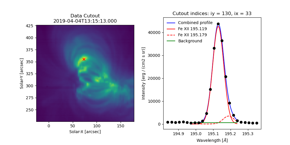
Complete example demonstrating reading data, slicing an EISCube, fitting the spectra, extracting the profile at the coordinates of maximum intensity, and finally making a nice overview plot.

import numpy as np
import matplotlib.pyplot as plt
import astropy.units as u
from astropy.coordinates import SkyCoord
from astropy.wcs.utils import wcs_to_celestial_frame
import eispac

if __name__ == '__main__':
    # Read in the fit template and EIS observation
    data_filepath = './eis_20190404_131513.data.h5'
    template_filepath = './fe_12_195_119.2c.template.h5'
    tmplt = eispac.read_template(template_filepath)
    data_cube = eispac.read_cube(data_filepath, tmplt.central_wave)

    # Select a cutout of the raster
    eis_frame = wcs_to_celestial_frame(data_cube.wcs)
    lower_left = [None, SkyCoord(Tx=-25, Ty=225, unit=u.arcsec, frame=eis_frame)]
    upper_right = [None, SkyCoord(Tx=175, Ty=425, unit=u.arcsec, frame=eis_frame)]
    raster_cutout = data_cube.crop(lower_left, upper_right)

    # Fit the data and save it to disk
    fit_res = eispac.fit_spectra(raster_cutout, tmplt, ncpu='max')
    save_filepaths = eispac.save_fit(fit_res, save_dir='cwd')

    # Find indices and world coordinates of max intensity
    sum_data_inten = raster_cutout.sum_spectra().data
    iy, ix = np.unravel_index(sum_data_inten.argmax(), sum_data_inten.shape)
    ex_world_coords = raster_cutout.wcs.array_index_to_world(iy, ix, 0)[1]
    y_arcsec, x_arcsec = ex_world_coords.Ty.value, ex_world_coords.Tx.value

    # Extract data profile and interpolate fit at higher spectral resolution
    data_x = raster_cutout.wavelength[iy, ix, :]
    data_y = raster_cutout.data[iy, ix, :]
    data_err = raster_cutout.uncertainty.array[iy, ix, :]
    fit_x, fit_y = fit_res.get_fit_profile(coords=[iy,ix], num_wavelengths=100)
    c0_x, c0_y = fit_res.get_fit_profile(0, coords=[iy,ix], num_wavelengths=100)
    c1_x, c1_y = fit_res.get_fit_profile(1, coords=[iy,ix], num_wavelengths=100)
    c2_x, c2_y = fit_res.get_fit_profile(2, coords=[iy,ix], num_wavelengths=100)

    # Make a multi-panel figure with the cutout and example profile
    fig = plt.figure(figsize=[10,5])
    plot_grid = fig.add_gridspec(nrows=1, ncols=2, wspace=0.3)

    data_subplt = fig.add_subplot(plot_grid[0,0])
    data_subplt.imshow(sum_data_inten, origin='lower', extent=cutout_extent)
    data_subplt.scatter(x_arcsec, y_arcsec, color='r', marker='x')
    data_subplt.set_title('Data Cutout\n'+raster_cutout.meta['mod_index']['date_obs'])
    data_subplt.set_xlabel('Solar-X [arcsec]')
    data_subplt.set_ylabel('Solar-Y [arcsec]')

    profile_subplt = fig.add_subplot(plot_grid[0,1])
    profile_subplt.errorbar(data_x, data_y, yerr=data_err, ls='', marker='o', color='k')
    profile_subplt.plot(fit_x, fit_y, color='b', label='Combined profile')
    profile_subplt.plot(c0_x, c0_y, color='r', label=fit_res.fit['line_ids'][0])
    profile_subplt.plot(c1_x, c1_y, color='r', ls='--', label=fit_res.fit['line_ids'][1])
    profile_subplt.plot(c2_x, c2_y, color='g', label='Background')
    profile_subplt.set_title(f'Cutout indices: iy = {iy}, ix = {ix}')
    profile_subplt.set_xlabel('Wavelength [$\AA$]')
    profile_subplt.set_ylabel('Intensity ['+raster_cutout.unit.to_string()+']')
    profile_subplt.legend(loc='upper left', frameon=False)
    plt.show()