Exploring EIS data

Once installed, EISPAC can be imported into any Python script or interactive session with a simple import eispac statement.

Reading Data into Python

Assuming you have already downloaded some data, the following code snippet below illustrates how to how to read the level-1 data from the spectral window containing the 195.12 Å line (window 7, in our example file). At the end of the chapter we will show how to examine a data header file to determine what wavelengths are available in a given observation.

>>> import eispac
>>> data_filename = 'eis_20190404_131513.data.h5'
>>> data_cube = eispac.read_cube(data_filename, 195.119)

The read_cube() function will read and apply all of the calibration and pointing corrections necessary for scientific analysis. The function has three key arguments (see the full documentation for additional keywords for specifying your own calibration curve or a count offset):

• filename (str or pathlib path) - Name or path of either the data or head HDF5 file for a single EIS observation

• window (int or float, optional) - Requested spectral window number (if <= 24) or the value of any wavelength within the requested window (in units of [Angstrom]). Default is “0”

• apply_radcal (bool, optional) - If set to True, will apply the pre-flight radiometric calibration curve found in the HDF5 header file and set units to \(erg/(cm^2 s sr)\). If set to False, will simply return the data in units of photon counts. Default is True.

EISCube Objects

The return value of read_cube is an EISCube class instance which contains calibrated intensities (or photon counts), corrected wavelengths, and all of the associated metadata. EISCube objects are a subclass of NDCube (from the Sunpy-affiliated package of the same name) and, as such, have built-in slicing and coordinate conversion capabilities as virtue of having an associated World Coordinate System (WCS) object.

The EISCube subclass extends ndcube by including a few additional features. First, an extra .wavelength attribute has been added which contains a 3D array with the corrected wavelength values at all locations within the cube. This correction accounts for two effects (1) a systematic spectral shift caused by a tilt in the orientation of the the EIS slit relative to the CCD and (2) a variable spectral shift caused by the orbit of the spacecraft. Secondly, four methods are included to quickly perform common EIS image manipulations,

• The apply_radcal and remove_radcal methods can be used to convert the data and uncertainty values to and from intensity and photon count units using either the pre-flight radiometric calibration curve provided in the HDF5 header file (default) or a user-inputted array. If apply_radcal is given a custom calibration curve, the number of data points in the input array must match the number of data points along the wavelength axis.

• The sum_spectra method sums the data along the wavelength axis and returns a new, 2D NDCube with just the data (no uncertainty or wavelength information). It requires no arguments.

• The smooth_cube method applies a boxcar moving average to the data along one or more spatial axes. It requires a single argument, “width”, that must be either a singular value or list of ints, floats, or astropy.units.Quantity instances specifying the number of pixels or angular distance to smooth over. If given a single value, only the y-axis will be smoothed. Floats and angular distances will be converted to the nearest whole pixel value. If a width value is even, width + 1 will be used instead. smooth_cube also accepts any number of optional keyword arguments that will be passed to the astropy.convolution.convolve function, which does the actual smoothing operation.

The calibrated intensity and uncertainty values are stored in numpy arrays in the .data and .uncertainty attributes. The order of the axes are (slit position, raster step, dispersion) which correspond to the physical axes of (Solar-Y, Solar-X, Wavelength). You can inspect the dimensions of an NDCube object like so,

>>> data_cube.dimensions
[512, 87, 24] pix

As you can see, our example data has dimensions of (512, 87, 24). That is, 512 pixels along the slit (in the Solar-Y direction), 87 raster steps (along the Solar-X axis), and 24 pixels along the dispersion (wavelength) axis.

Slicing an EISCube

One of the most powerful features of NDCube-based objects is the ability to slice using either array indices or world coordinates. Slicing by array indices works just like slicing a normal numpy array. Slicing by coordinates is done using the ndcube.NDCube.crop method and a collection of two or more points constructed using high level coordinate objects from astropy.coordinates. Note: for spatial coordinates, you must specify the observer frame, which can be constructed using the EISCube.wcs object.

For example,

>>> import astropy.units as u
>>> from astropy.coordinates import SkyCoord, SpectralCoord
>>> from astropy.wcs.utils import wcs_to_celestial_frame
>>> eis_frame = wcs_to_celestial_frame(data_cube.wcs)
>>> lower_left = [SpectralCoord(195.0, unit=u.angstrom),
...               SkyCoord(Tx=48, Ty=225, unit=u.arcsec, frame=eis_frame)]
>>> upper_right = [SpectralCoord(195.3, unit=u.AA),
...                SkyCoord(Tx=165, Ty=378, unit=u.arcsec, frame=eis_frame)]
>>> data_cutout = data_cube.crop(lower_left, upper_right)
>>> data_cutout.dimensions
[154, 48, 14] pix

Slicing an EISCube also automatically slices all of the associated subarrays (data, uncertainty, wcs, and wavelength). Please see the ndcube documentation for more information about slicing and manipulating NDCube objects.

Attention

Slicing the wavelength axis with .crop() uses the wavelength values in the WCS object, NOT the corrected values stored in .wavelength. Please use with care. If you don’t want or need to slice along the wavelength axis, simply give the function a value of None instead of a SpectralCoord object.

Exploring Metadata

All metadata and information from the HDF5 header file are packed into a single dictionary stored in the .meta attribute of the EISCube. The structure of the .meta dictionary mirrors the internal structure of the HDF5 file, with a few extra keys added for convenience. You can explore the contents with the usual Python commands,

>>> data_cube.meta.keys()
dict_keys(['filename_data', 'filename_head', 'wininfo', 'iwin', 'iwin_str',
           'index', 'pointing', 'wave', 'radcal', 'slit_width',
           'slit_width_units', 'ccd_offset', 'wave_corr', 'wave_corr_t',
           'wave_corr_tilt', 'date_obs', 'date_obs_format', 'duration',
           'duration_units', 'mod_index', 'aspect', 'aspect_ratio', 'notes'])
>>> data_cube.meta['pointing']['x_scale']
2.9952
>>> data_cube.meta['radcal']
array([8.06751  , 8.060929 , 8.054517 , 8.048271 , 8.042198 , 8.036295 ,
       8.030562 , 8.024157 , 8.017491 , 8.010971 , 8.0046015, 7.998385 ,
       7.9923196, 7.9864078, 7.980654 , 7.975055 , 7.969617 , 7.9643393,
       7.959224 , 7.9542727, 7.949487 , 7.9448686, 7.9404206, 7.9361415],
      dtype=float32)

Assorted metadata

For completeness and transparency, we have bundled all of the commonly used instrumental and processing metadata provided in IDL. EISPAC attempts to correct for most instrumental effects, so you will not need to reference the ccd_offset or wave_corr_tilt, for example, but that information is there if you want it. As a reminder, the slit_width array gives the empirically-determined instrumental broadening along the EIS slit, and not the physical width of the slit itself.

Here x_scale is the number of arcsec between step positions in the raster. Most EIS rasters take more than 1 arcsec per step, which degrades the spatial resolution but increases the cadence. The variable radcal is the pre-flight calibration curve for this data window. It includes all of the factors for converting counts directly to \(erg/(cm^2 s sr)\).

Of particular note, the .meta['index'] dictionary contains the original EIS Level-0 FIT header keywords. Be aware, the pointing information in the Level-0 header is uncorrected. The .meta['mod_index'] (modified index) dictionary contains a reduced set of header keywords including all pointing corrections. Additionally, the mod_index values are updated by EISPAC whenever the EISCube is sliced while the original index is not updated.

Spectral Windows

We usually don’t care about the numbering of the data windows. It’s more natural to want to read the data corresponding to a particular wavelength. The read_wininfo function can be used help identify the spectral contents of each data window. The function takes an input header file and returns a numpy.recarray containing the window numbers, min and max wavelengths and primary spectral line for each data window. Note: for your convenience, a copy of the wininfo array is also stored in the EISCube.meta dictionary.

>>> import eispac
>>> header_filename = 'eis_20190404_131513.head.h5'
>>> wininfo = eispac.read_wininfo(header_filename)
>>> wininfo.dtype.names
('iwin', 'line_id', 'wvl_min', 'wvl_max', 'nl', 'xs')
>>> wininfo[0:4]
rec.array([(0, 'Fe XI 180.400', 180.03426, 180.72559, 32, 661),
           (1, 'Ca XV 182.100', 181.75139, 182.44266, 32, 738),
           (2, 'Fe X 184.720', 183.82512, 185.5865 , 80, 831),
           (3, 'Fe XII 186.750', 186.3891 , 187.0802 , 32, 946)],
           ... ... ...
           (23, 'Mg VII 280.390', 279.7766 , 280.9996 , 56, 3720),
           (24, 'Fe XV 284.160', 283.89   , 284.40134, 24, 3905)],
          dtype=[('iwin', '<i4'), ('line_id', '<U64'), ('wvl_min', '<f4'),
                 ('wvl_max', '<f4'), ('nl', '<i4'), ('xs', '<i4')])

We can then use a numpy.where call on the wininfo array to map wavelength to window number. Users familiar with IDL may be interested to note that numpy record arrays can be accessed like an IDL array of structures (e.g. instead of wininfo['wvl_min'] below, you could also use wininfo.wvl_min).

>>> import numpy as np
>>> wvl = 195.119
>>> p = (wininfo['wvl_max'] - wvl)*(wvl - wininfo['wvl_min'])
>>> iwin = np.where(p >= 0)[0]
>>> iwin
array([7], dtype=int64)

If the result is an empty array, the wavelength is not in the data.

Plotting

We can make a quick image of the EIS data by making use of the .plot() method provided in all NDCube objects (note, it usually helps to sum along the dispersion direction first).

>>> data_cube.sum_spectra().plot(aspect=data_cube.meta['aspect'])

The .plot() method can also be used to display the spectrum from a single pixel, as shown below. For illustration, we also convert the data back in units of photon counts (this is the same as dividing the calibrated data by the .meta['radcal'] array).

>>> ix = 48
>>> iy = 326
>>> spec = data_cube[iy,ix,:].remove_radcal()
>>> spec_plot = spec.plot()
>>> spec_plot.set_title(f'ix = {ix}, iy = {iy}, units = counts')

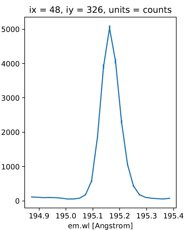
Fig. 3 An example Fe XII 195.119 Å line profile from the raster.

To perform more advanced plotting, such as logarithmically scaling the intensities, you will need to extract the data from the EISCube and create the figure yourself using any of the various Python plotting libraries. For example,

import numpy as np
import matplotlib.pyplot as plt
import eispac

data_filename = 'eis_20190404_131513.data.h5'
data_cube = eispac.read_cube(data_filename, 195.119)
raster_sum = np.sum(data_cube.data, axis=2) # or data_cube.sum_spectra().data
scaled_img = np.log10(raster_sum)

plt.figure()
plt.imshow(scaled_img, origin='lower', extent=data_cube.meta['extent_arcsec'], cmap='gray')
plt.title(data_cube.meta['date_obs'][-1])
plt.xlabel('Solar-X [arcsec]')
plt.ylabel('Solar-Y [arcsec]')
plt.show()

Tip

Setting both “aspect” (y_scale/x_scale) and “extent” (data range as [left, right, bottom, top]) in plt.imshow() can sometimes give unexpected results. You may need to experiment with the combination of keywords needed to get the plot you expect.

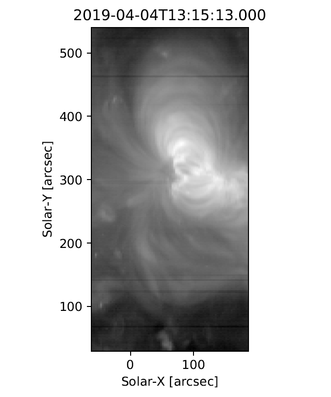
Fig. 4 An example image formed by summing the data for the Fe XII spectral window in the dispersion direction. In a subsequent chapter we’ll discuss fitting the spectra.

Footnotes

[1]

The .crop() method was added in NDCube 2.0. In older versions of the code (before 2021-10-29), there was a method called .crop_by_coords which worked slightly differently.