Fitting the Data

Why use MPFIT?

We have chosen to use MPFIT due to its flexibility and long (20+ year) legacy in solar and heliophysics. While newer fitting methods provide powerful tools for data exploration, they are still young and incur significant additional computation time (and are also more complicated to parallelize).

Fitting of the spectra involves selecting a spectral line of interest (e.g. 195.119 Å) from one of the spectral windows of in the data, choosing a function (or combination of functions) to fit, and determining an initial guess for each parameter. The next ingredient for a fit is the selection of an optimization method. By default, EISPAC uses a Python implementation of the well-known IDL method MPFIT, which solves the non-linear least squares problem using the Levenberg- Marquardt algorithm. The Python module, mpfit.py, is included in EISPAC and the orginal source code can found on GitHub [1]. Future versions of of EISPAC may include support for other fitting packages such as the newer astropy.modeling framework.

Template Files

In order to make fitting quick and easy, we’ve created a set of fit templates for different spectral lines. Each template consists of one or more component Gaussian functions and a constant background term. Template files are named according to the following pattern: {primary spectral line}.{number of Gaussians}c.template.h5. 119 templates are provided with EISPAC, covering all of the commonly observed spectral line combinations.

The easiest way to browse and copy fit template files is to use the eis_browse_templates GUI tool included with EISPAC. This tool can be used to display a list of all templates available for each spectral window in an EIS observation and copy the template files to your work directory (see the eis_browse_templates section for a few tips). A similar result can be obtained with the match_templates function, which takes either an EISCube or the path to a header file and outputs a list (or list of lists) of all fit templates available for a given spectral window (or data file).

>>> import eispac
>>> data_filename = 'eis_20190404_131513.data.h5'
>>> data_cube = eispac.read_cube(data_filename, 195.119)
>>> template_list = eispac.match_templates(data_cube)
>>> for file in template_list:
>>>     print(file.name)
fe_12_195_119.1c.template.h5
fe_12_195_119.2c.template.h5
fe_12_195_179.2c.template.h5

In the example above, notice how both one and two component fits are available for the same line. Furthermore, as with many multi-component templates, the third template file is actually a duplicate of the second template, just with the name of the secondary spectral line in the filename. This was designed to make it easier to see exactly which spectral lines can be fit. However, it also means you cannot simply loop over all template files available for a given spectral window, as you would be unnecessarily multiplying the amount of fitting performed (and resultant output files).

We recommend copying the template files you wish to use to your project directory so you have a more self-contained record of your fitting process. Assuming you are running Python from your project directory, the following code snippet illustrates one method you could use.

>>> import os
>>> import shutil
>>> current_dir = os.getcwd()
>>> shutil.copy(template_list[1], current_dir)

Attention

Take care to only copy template files. Moving a template from your EISPAC installation will lead to incomplete results in future calls to match_templates().

Loading Fit Templates

An h5dump [2] on one of the template files shows that it contains a /template group for the initial guess on the fit parameters and a /parinfo group containing constraints on the parameters for use by mpfit.

h5dump -n fe_12_195_119.2c.template.h5
HDF5 "fe_12_195_119.2c.template.h5" {
FILE_CONTENTS {
 group      /
 group      /parinfo
 dataset    /parinfo/fixed
 dataset    /parinfo/limited
 dataset    /parinfo/limits
 dataset    /parinfo/tied
 dataset    /parinfo/value
 group      /template
 dataset    /template/component
 dataset    /template/data_e
 dataset    /template/data_x
 dataset    /template/data_y
 dataset    /template/fit
 dataset    /template/fit_back
 dataset    /template/fit_gauss
 dataset    /template/line_ids
 dataset    /template/n_gauss
 dataset    /template/n_poly
 dataset    /template/order
 dataset    /template/wmax
 dataset    /template/wmin
 }

The read_template function can be used to read a template file and examine the contents.

>>> import eispac
>>> tmplt_filename = 'fe_12_195_119.2c.template.h5'
>>> tmplt = eispac.read_template(tmplt_filename)

Use the command print(TEMPLATE) to view a summary of the template, intial parameter values, and constraints in a nice format.

>>> print(tmplt)
--- EISFitTemplate SUMMARY ---
filename_temp: ./fe_12_195_119.2c.template.h5
n_gauss: 2
n_poly: 1
line_ids: ['Fe XII 195.119' 'Fe XII 195.179']
wmin, wmax: 194.9600067138672, 195.25

--- PARAMETER CONSTRAINTS ---
 *            Value   Fixed     Limited              Limits                Tied
p[0]     57514.6647       0     1     0       0.0000       0.0000
p[1]       195.1179       0     1     1     195.0778     195.1581
p[2]         0.0289       0     1     1       0.0191       0.0510
p[3]      8013.4013       0     1     0       0.0000       0.0000
p[4]       195.1779       0     1     1     195.1378     195.2181          p[1]+0.06
p[5]         0.0289       0     1     1       0.0191       0.0510          p[2]
p[6]       664.3349       0     0     0       0.0000       0.0000

funcinfo dictionary

The EISFitTemplate object returned by eispac.read_template() also generates a .funcinfo list. This list will help with the implementation of other fitting methods in the future, but is currently not used by the code and can, thereby, be safely ignored.

The structure of parinfo is specific to MPFIT and should be familiar to anyone who has used the original IDL version; please see the section on Constraining Parameter Values for more details. The templates provided with EISPAC consist of one or more Gaussian functions (with parameters in the order of peak, centroid, & width) followed by one or more background polynomial terms (usually just a single, constant value). The values .template['n_gauss'] and .template['n_poly'] indicate, respectively, the number of Gaussian functions and background polynomial terms in a given template.

Note

The multigaussian function is composed of generalized Gaussian functions of the form \(f(x) = A exp(-(x-b)^2/2c^2)\), where A is the amplitude (peak value), b is the position of the center of the peak (centroid), and c is the standard deviation (width). This is consistent with the fit parameters used for EIS data in the IDL SolarSoftWare (SSW) analysis suite.

Custom Fit Templates

EISPAC comes with a wide selection of templates that cover the most common EIS lines. However, you can also define a custom fitting template for more specific use-cases. There are two initialization methods available. First, you can call the EISFitTemplate class directly and pass in the appropriate values and arrays. Here is an example for initializing a template with a single Gaussian function and constant background.

>>> new_tmplt = eispac.EISFitTemplate(value=[57514.7, 195.1, 0.0289, 664.3], line_ids=['Fe XII 195.119'])

At minimum, you need to provide a value list or array giving the initial values for each fitting parameter. The order of parameters is assumed to be sets of [PEAK, CENTROID, WIDTH] for each Gaussian component followed, optionally, by the coefficients the background polynomial, starting with the LOWEST (constant) order term first. If only a value array is provided (as in the example above), the code will estimate the number of Gaussians and polynomial terms based on the total number of parameters. Other valid template keys include,

• n_gauss (int) - number of Gaussian components

• n_poly (int) - Number of background polynomial terms. Common values are: 0 (no background), 1 (constant), and 2 (linear).

• line_ids (array-like) - Strings giving the line identification

  for each Gaussian component. For example, “Fe XII 195.119”. If not specified, placeholder values of “unknown I {INITAL CENTROID VALUE}” will be used.

• wmin and wmax (floats) - min and max wavelength value of data to use for fitting. Any data in the window outside the range delimited by these two keys will be ignored during fitting.

The following keys are all additional parameter constraints that will be stored in the .parinfo list of dicts. As such, they must be input as arrays or lists with the same number of elements as the value array.

• fixed (0 or 1) - If set to “1”, will not fit the parameter and just use initial value instead

• limited (two-element array-like) - If set to “1” in the first/second value, will apply and limit to the parameter on the lower/upper side

• limits (two-element array-like) - Values of the limits on the lower/upper side. Both “limited” and “limits” must be give together.

• tied (str) - String defining a fixed relationship between this parameters one or more others. For example “p[0] / 2” would define a parameter to ALWAYS be exactly half the value of the first parameter.

The second method for initializing a custom template is to write a separate TOML-formatted text file with all of the input parameters and then load the custom template file using the read_template. This allows you to save, reuse, and share your templates without needing to copy/paste Python code. Please note: there is currently no function to export a template from EISPAC and save it to a TOML file; you will need to create the TOML file yourself using your favorite text editor. Below is an example TOML file with a copy of the two-component Fe XII 195.119 template provided with EISPAC.

[template]
n_gauss = 2
n_poly = 1
line_ids = ['Fe XII 195.119', 'Fe XII 195.179']
wmin = 194.96
wmax = 195.25

[parinfo]
value = [
   57514.6647, 195.1179, 0.0289,
   8013.4013, 195.1779, 0.0289,
   664.3349
]
fixed = [0,0,0,0,0,0,0]
limited = [[1,0],[1,1],[1,1],[1,0],[1,1],[1,1],[0,0]]
limits = [
   [1,0],[195.0778,195.1581],[0.0191,0.0510],
   [1,0],[195.1378,195.2181],[0.0191,0.0510],
   [1,0]
]
tied = ['', '', '', '', 'p[1]+0.06', 'p[2]', '']

Assuming this was saved in a file named “custom_fe_12_195.toml”, you can then easily load it in using the command fe_12_tmplt = eispac.read_template(“custom_fe_12_195.toml”). For more information about TOML files, please see the official documentation

Fitting Spectra

Once you’ve read in a template file, you can use the central wavelength to find the desired spectral window in the data using read_cube.

>>> data_filename = 'eis_20190404_131513.data.h5'
>>> data_cube = eispac.read_cube(data_filename, tmplt.central_wave)

As mentioned in the previous chapter, read_cube automatically applies all of the pointing and wavelength corrections, bad data masking, and error estimations needed for scientific analysis. By default, the code also converts the data from photon counts to intensity units of erg cm\(^{-2}\) s\(^{-1}\) sr\(^{-1}\) using the appropriate pre-flight calibration curve. This conversion can be disabled by setting the keyword apply_radcal=False, should you prefer to run your fits in count space.

Summary of fitting process

Here’s what’s happening under the hood, fit_spectra() calls the helper function scale_guess() to scale the initial parameter values to the data, then mpfit is called to actually run the Levenberg-Marquardt fitting on a custom function that computes the deviates between the input spectrum and a multigaussian fit. If ncpu is set to a value > 1, then each raster step position will be processed separately and the full set of results will be combined into a single output.

On to the fitting! Now that you have a template and the data elements, you can perform a fit of the entire data cube by calling the top-level fitting routine, fit_spectra. The easiest way to use fit_spectra is to just give it both an EISCube and EISFitTemplate object (or filepaths to the data and template HDF5 files). You may slice your EISCube however you wish before fitting and the code will loop over the data appropriately (this includes fitting a single spectra or slit observation). Additionally, fit_spectra takes advantage of the multiprocessing package in the Python standard library to automatically parallelize the fitting process and minimize the run time. You may control the number of processing cores used for the fitting with ncpu keyword, or set it equal to “max” or None to use the maximum number of cores available. Please see the full doc string for fit_spectra for additional options and parameters.

Attention

Due to the specifics of how the multiprocessing library works, any statements that call fit_spectra() using ncpu > 1 MUST be wrapped in a "if __name__ == __main__:" statement in the top-level script or program. If such a “name guard” statement is not detected, fit_spectra() will fall back to using a single process. Unfortunately, this means you can not directly use parallel fitting from an interactive Python shell, you must first write a program that you save and run.

Here is a minimal example program that just loads and fits the data.

import eispac

if __name__ == '__main__':
    # input data and template files
    data_filepath = './eis_20190404_131513.data.h5'
    template_filepath = './fe_12_195_119.2c.template.h5'

    # read fit template
    tmplt = eispac.read_template(template_filepath)

    # Read spectral window into an EISCube
    data_cube = eispac.read_cube(data_filepath, tmplt.central_wave)

    # Fit the data, then save it to disk and test loading it back in
    fit_res = eispac.fit_spectra(data_cube, tmplt, ncpu='max')
    save_filepaths = eispac.save_fit(fit_res, save_dir='cwd')
    FITS_file = eispac.export_fits(fit_res, save_dir='cwd')
    load_fit = eispac.read_fit(save_filepaths[0])

Note

The command line script eis_fit_files can be used to quickly fit a directory of files using one or more templates in another directory.

EISFitResult Objects

fit_spectra outputs an EISFitResult object, which may be saved to an HDF5 file and read back in later using the save_fit and read_fit functions (as shown in the example above). The output fit parameters are stored in a dictionary of arrays.

>>> for key in fit_res.fit.keys():
...     print(f"{key:<15} {fit_res.fit[key].dtype} {fit_res.fit[key].shape}")

line_ids        <U14 (2,)
main_component  int16 ()
n_gauss         int16 ()
n_poly          int16 ()
wave_range      float64 (2,)
status          float64 (128, 32)
chi2            float64 (128, 32)
mask            int32 (128, 32, 24)
wavelength      float64 (128, 32, 24)
int             float64 (128, 32, 2)
err_int         float64 (128, 32, 2)
vel             float64 (128, 32, 2)
err_vel         float64 (128, 32, 2)
width           float64 (128, 32, 2)
err_width       float64 (128, 32, 2)
params          float64 (128, 32, 7)
perror          float64 (128, 32, 7)
component       int32 (7,)
param_names     <U32 (7,)
param_units     <U32 (7,)

We can extract an array of the fit parameters or intensity profile using the get_params and get_fit_profile methods. Both methods take optional keywords for selecting the component number and/or an individual pixel (using array coordinates). get_fit_profile also has a num_wavelengths keyword that allows us to interpolate the fit profile at a higher wavelength resolution than observed by EIS. The use of these methods are demonstrated in the longer example program below, which also shows one method for finding the indices and coordinates of maximum intensity.

import numpy as np
import matplotlib.pyplot as plt
import astropy.units as u
from astropy.coordinates import SkyCoord
from astropy.wcs.utils import wcs_to_celestial_frame
import eispac

if __name__ == '__main__':
    # Read in the fit template and EIS observation
    data_filepath = './eis_20190404_131513.data.h5'
    template_filepath = './fe_12_195_119.2c.template.h5'
    tmplt = eispac.read_template(template_filepath)
    data_cube = eispac.read_cube(data_filepath, tmplt.central_wave)

    # Select a cutout of the raster
    eis_frame = wcs_to_celestial_frame(data_cube.wcs)
    lower_left = [None, SkyCoord(Tx=-25, Ty=225, unit=u.arcsec, frame=eis_frame)]
    upper_right = [None, SkyCoord(Tx=175, Ty=425, unit=u.arcsec, frame=eis_frame)]
    raster_cutout = data_cube.crop(lower_left, upper_right)

    # Fit the data and save it to disk
    fit_res = eispac.fit_spectra(raster_cutout, tmplt, ncpu='max')
    save_filepaths = eispac.save_fit(fit_res, save_dir='cwd')

    # Find indices and world coordinates of max intensity
    sum_data_inten = raster_cutout.sum_spectra().data
    iy, ix = np.unravel_index(sum_data_inten.argmax(), sum_data_inten.shape)
    ex_world_coords = raster_cutout.wcs.array_index_to_world(iy, ix, 0)[1]
    y_arcsec, x_arcsec = ex_world_coords.Ty.value, ex_world_coords.Tx.value

    # Extract data profile and interpolate fit at higher spectral resolution
    data_x = raster_cutout.wavelength[iy, ix, :]
    data_y = raster_cutout.data[iy, ix, :]
    data_err = raster_cutout.uncertainty.array[iy, ix, :]
    fit_x, fit_y = fit_res.get_fit_profile(coords=[iy,ix], num_wavelengths=100)
    c0_x, c0_y = fit_res.get_fit_profile(0, coords=[iy,ix], num_wavelengths=100)
    c1_x, c1_y = fit_res.get_fit_profile(1, coords=[iy,ix], num_wavelengths=100)
    c2_x, c2_y = fit_res.get_fit_profile(2, coords=[iy,ix], num_wavelengths=100)

    # Make a multi-panel figure with the cutout and example profile
    fig = plt.figure(figsize=[10,5])
    plot_grid = fig.add_gridspec(nrows=1, ncols=2, wspace=0.3)

    data_subplt = fig.add_subplot(plot_grid[0,0])
    data_subplt.imshow(sum_data_inten, origin='lower', extent=cutout_extent)
    data_subplt.scatter(x_arcsec, y_arcsec, color='r', marker='x')
    data_subplt.set_title('Data Cutout\n'+raster_cutout.meta['mod_index']['date_obs'])
    data_subplt.set_xlabel('Solar-X [arcsec]')
    data_subplt.set_ylabel('Solar-Y [arcsec]')

    profile_subplt = fig.add_subplot(plot_grid[0,1])
    profile_subplt.errorbar(data_x, data_y, yerr=data_err, ls='', marker='o', color='k')
    profile_subplt.plot(fit_x, fit_y, color='b', label='Combined profile')
    profile_subplt.plot(c0_x, c0_y, color='r', label=fit_res.fit['line_ids'][0])
    profile_subplt.plot(c1_x, c1_y, color='r', ls='--', label=fit_res.fit['line_ids'][1])
    profile_subplt.plot(c2_x, c2_y, color='g', label='Background')
    profile_subplt.set_title(f'Cutout indices: iy = {iy}, ix = {ix}')
    profile_subplt.set_xlabel('Wavelength [$\AA$]')
    profile_subplt.set_ylabel('Intensity ['+raster_cutout.unit.to_string()+']')
    profile_subplt.legend(loc='upper left', frameon=False)
    plt.show()

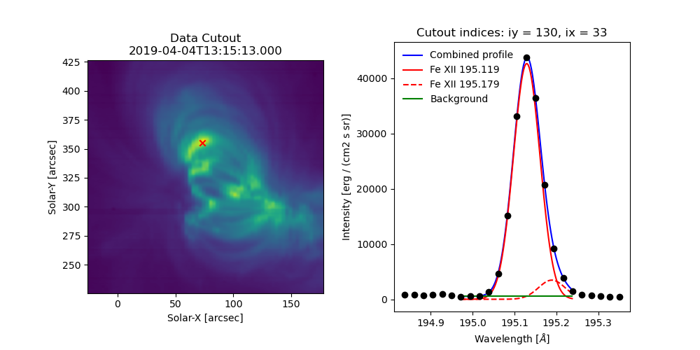
Fig. 5 Example data cutout (left) and fit profile (right) for the spectral window containing the Fe XII 195.119 Å line. The red X shows the location of the maximum summed intensity.

EISMaps for Sunpy

The fit line intensities, velocities, and widths can be loaded into an EISMap, which is a subclass of sunpy.map.Map. This allow us to leverage the full power of Sunpy to do all sorts of cool science like comparing spacecraft locations, co-aligning images, reprojecting maps, and performing field extrapolations (see the Map sections of the SunPy User’s Guide and Example Gallery for some demonstrations). You can get an EISMap by either using the get_map method or saving the measurements to FITS files using export_fits and then loading them in with either eispac.EISMap(FILENAME) or even sunpy.map.Map(FILENAME) (assuming EISPAC is also imported in your program).

For now, we will just show you some examples of the quick-look plots.

>>> # Fit intensity (in a nice sunpy Map)
>>> inten_map = fit_res.get_map(component=0, measurement='intensity')
>>> inten_map.peek()

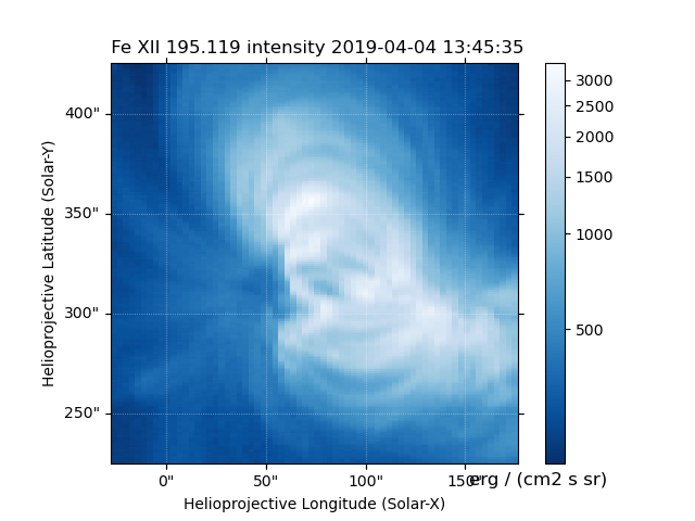
Fig. 6 Fit line intensity in a nice SunPy Map.

>>> # Fit velocity map
>>> # Note: You can also use positional arguments and abbreviations
>>> vel_map = fit_res.get_map(0, 'vel')
>>> vel_map.peek()

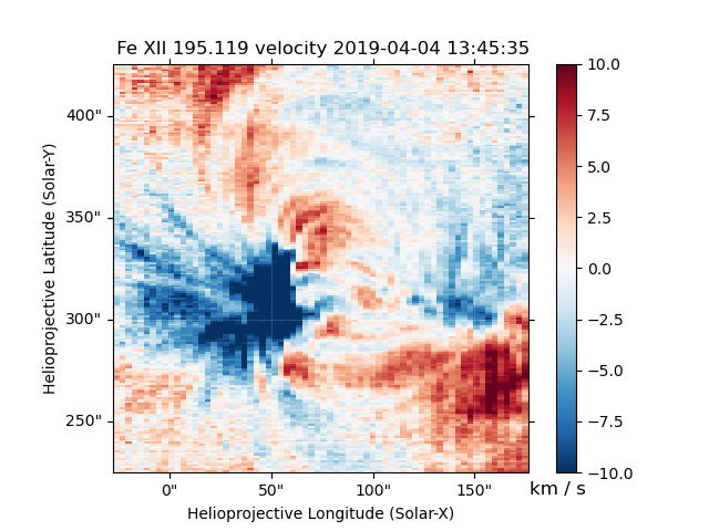
Fig. 7 Fit line velocity map.

Attention

While we have corrected the velocity maps for orbital effects, there are still some unknown uncertainties. This is largely the case for ALL EIS velocity maps, not just those computed by EISPAC. Please use with care.

Footnotes

[1]

Sergey Koposov’s Python port of MPFIT can be found at https://github.com/segasai/astrolibpy/

[2]

h5dump is a command line tool used to inspect the contents of an HDF5 file. It is included the Anaconda Python distribution platform, but can also be installed on its own.